An Adversarial (re)Analysis of Zhou/Firestone 2019
This post is a reanalysis of Zhenglong Zhou and Chaz Firestone’s paper “Humans can deciper adversarial images,” so let’s get some links out of the way
- Paper - Zhou Z, Firestone C. Humans can deciper adversarial images. Nature Communications 10(1):1334 p.2041-1723, DOI:10.1038/s41467-019-08931-6
- Preprint
- Data and Code on OSF
Overview
Chaz Firestone came and presented this data at the UO’s cognitive neuroscience seminar series this winter just before the paper came out. The idea is compelling: Convolutional neural nets trained to classify images are vulnerable to adversarial attacks where images can be manipulated or synthesized to trigger a specific categorization.
On their face, these adversarial images highlight the dramatic differences between the human/mammalian visual system – the types of things that fool us are very different than tactically adding static throughout an image. However if there were any overlap between the types of adversarial image manipulations that fool us and fool CNNs, they argue it would point to a possible mechanistic overlap.
They use two types of adversarial images:
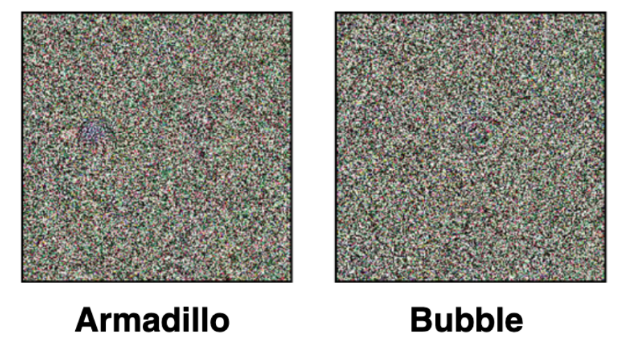
Fooling images are otherwise meaningless patterns that are classified as familiar objects by a machine-vision system.
 ya fooled me doc
and
Perturbed images are images that would normally be classified accurately and straightforwardly […] but that are perturbed only slightly to produce a completely different classification by the machine
 youch wat trickery!
They present 8 experiments with 5 image sets that mostly ask human subjects to guess what a computer would classify the images as – what they call “machine theory of mind” – although the degree to which that is different than just having people classify images is ambiguous in their data.
Clarifying Hypotheses
There seems to be an abnormally high airgap between data and interpretation here that I think is worthy of careful handling. The ultimate motivation here is to detect some similarity between CNNs and mammalian/human visual systems, and since CNNs seem to be vulnerable to adversarially manipulated images, if there is mechanistic overlap humans should be too. The authors aim to fill the empirical gap where, according to them, no one has actually tested whether humans misclassify these images
A primary factor that makes adversarial images so intriguing is the intuitive assumption that a human would not classify the image as the machine does. (Indeed, this is part of what makes animage“adversarial”in thefirst place, though that definition is notyet fully settled.) However, surprisingly little work has actively explored this assumption by testing human performance on such images, even though it is often asserted that adversarial images are “totally unrecognizable to human eyes”
There are a number of very similar hypotheses and results that are possible here, we should delineate between them.
The most straightforward test of a hypothesis would be:
Base image, well classified by humans and CNNs -> Perturbed image, CNNs consistent misclassify -> If humans misclassify in the same way and at same rate, implied mechanistic similarity.
A critical component of this is that the image is misclassified according to humans, or classified in a way that is not “what is looks like.” There is a tautology that makes this experiment impossible (as the authors note) - if the adversarially manipulated image didn’t still “look like” the base image, it wouldn’t be an adversarially useful image. A less strong test of the hypothesis would be to relax the requirement that there be some well-classified base image
Generated or perturbed image not obviously classified by humans, CNNs consistently classify -> when forced, if humans classify in same way at same rate, implied mechanistic similarity. (similar to experiments 3a, 3b)
In this case, the images cannot obviously resemble the classes they are assigned by the CNN, as that would just mean the CNNs correctly learned some abstract representation of the way images look to humans. Such a result is not uninteresting, it is just the same as finding that CNNs can classify images, and we know that already. To the degree than an image resembles the class that the CNN assigned it, that image is not suitable to test this hypothesis. Another subtlety here is that the humans should have to classify in the same way as the CNNs, ie. choose from a list of all possible categories. Giving additional structure to the humans would require giving the same to the CNNs to make the results comparable.
There are several implicit hypotheses tested in this paper that are essentially unrelated to the central question of machine/human overlap.
Humans are told images were misclassified, choose the misclassification from an array of all possible image classes. If misclassification correctly identified, humans can recognize visual features that drive misclassifications in CNNs. (experiment 5)
This is a distinct hypothesis from ‘humans have the same visual processing as CNNs,’ in this case since the human subjects are told there is a misclassification, they are looking not for what they think the image actually is, but for what would have driven the mistake. The interpretation should be that humans are capable of inferring what makes a machine misclassify an image, not that we process images similarly.
Humans are given an image class and examples, if they choose the image that was categorized as that class, they can recognize some element of the image class in the adversarial image. (experiment 4)
This is another separate question – in this case the subjects are asked to recognize some feature from the example images in the perturbed images. Their being able to see those features is not indicative that they process the images in the same way as the CNN, but amongst an array of imperfect examples they can see the image that is the most similar to the example images.
The optimal outcome for all of these experiments is
- The subject all categorize with high accuracy - the subjects should all have the same performance as the machine to affirm the hypothesis.
- The images are all categorized with equal accuracy - since the question is about human/machine agreement in general, that overlap should be true of all images. Having images with wildly different accuracy rates is useful to assess the visual features that drive human/machine, but for the same reason points to some specific qualities of the images that make the more and less accurately categorized rather than a general similarity between human/machine overlap. Remember – the machines classify all of these images incorrectly with a high degree of confidence, so humans should too.
Reanalysis Details
Aside from the structure of the hypotheses, I had questions about the data analysis itself. During his presentation I was confused about why the data was reported as it was – the main results they report are the % of subjects whose categorization agreed with the machine and % of images where the majority categorization agreed with the machine. It seemed like that analysis would obscure the actual rates of categorization – ie. the actual rate of “correct” responses grouped by subject and image. The percents of subject and image agreement were also counted just by their mean categorization being above chance rather than being statistically distinguishable from chance (ie. confidence intervals exclude the chance threshold), I will also report those as “adjusted accuracies” using pearson-klopper binomial 95% confidence intervals.
Because I think this is such a potentially cool line of research I thought I would do the reanalysis myself. Thankfully, the authors released their (very clean!) data. I think the results are quite a bit more subtle than initially reported.
Code Boilerplate
We’ll use the following libraries
library(tidyverse)
library(lme4)
library(rio)
library(binom)
library(here)
library(caret)
I’ve put the data in a directory in my website structure, “/assets/data/adv”. We’ll load them all into variable names expt_1, expt_2, etc. and do some cleanup.
# list experiment data files
experiment_dirs <- list.dirs(here('assets', 'data', 'adv'), full.names=FALSE, recursive=FALSE)

# name each dataset according to its number
experiment_names <- c("expt_1", "expt_2", "expt_3a", "expt_3b", "expt_4", "expt_5", "expt_6", "expt_7")

# list the datafiles
data_files <- c()
for (i in seq(length(experiment_dirs))){
  data_files[i] <- list.files(here('assets', 'data', 'adv', experiment_dirs[i], "data"), full.names = TRUE)[1]
}

# load experiments
for (i in seq(length(data_files))){
  assign(experiment_names[i],
         as.tbl(import_list(data_files[i])$Data))
}

##########################
## clean data

# rename columns
names(expt_1)[c(1, 9, 10, 11)] <- c("subject", "correct", "rt_pass", "complete")
names(expt_2)[c(1, 9, 10, 11)] <- c("subject", "correct", "rt_pass", "complete")
names(expt_3a)[c(1, 6, 7, 8)] <- c("subject", "correct", "rt_pass", "complete")
names(expt_3b)[c(1, 6, 7, 8)] <- c("subject", "correct", "rt_pass", "complete")
names(expt_4)[c(1,6,7,8,9)] <- c("subject", "correct", "rt_pass", "rt_allpass", "complete")
names(expt_5)[c(1,7,8,9)] <- c("subject", "correct", "rt_pass",  "complete")
names(expt_6)[c(1,10,11,12)] <- c("subject", "correct", "rt_pass", "complete")
names(expt_7)[c(1,10,11,12)] <- c("subject", "correct", "rt_pass", "complete")

# retype columns
for (expt_name in experiment_names){
  # use get to refer to the object with its character name not its symbol name
  xpt <- get(expt_name)

    # subset incomplete subjects
  xpt <- xpt[xpt$complete == TRUE,]
  if ("rt_allpass" %in% names(xpt)){
    xpt <- xpt[xpt$rt_allpass==TRUE,]
  }

  # first columns present in all dfs
  xpt <- xpt %>% mutate(
    subject = as.factor(subject),
    correct = as.logical(correct),
    rt_pass = as.logical(rt_pass),
    complete = as.logical(complete)
  )

  # then specifics
  if ("image" %in% names(xpt)){
    xpt$image <- as.factor(xpt$image)
  }

  if ("response" %in% names(xpt)){
    xpt$response <- as.factor(xpt$response)
  }


  # assign back to name

  assign(expt_name,
         xpt)
}
Summarizing Functions
Since so much of the data has the same structure, we’ll write functions to summarize the image responses by image and subject. They’ll return
n_trials- the number of trials per groupn_correct- the number of “correct,” or matching the categorization of the CNN, trialsmeancx- the proportion of correct answers per groupcilo,cihi- the 95% confidence interval around the mean correct.
summarize_data <- function(data){

  summary_image <- data %>% group_by(image) %>%
  summarize(n_trials = length(correct),
            n_correct = sum(correct),
            meancx = n_correct/n_trials,
            meanrt = mean(rt),
            sdrt = sd(rt),
            cilo = binom.confint(sum(correct),length(correct),
                                  conf.level=0.95,method="exact")[[5]],
            cihi = binom.confint(sum(correct),length(correct),
                                  conf.level=0.95,method="exact")[[6]])

  summary_image$image <- ordered(summary_image$image,
                              levels=summary_image$image[order(summary_image$meancx)])

  summary_subject <- data %>% group_by(subject) %>%
    summarize(n_trials = length(correct),
              n_correct = sum(correct),
              meancx = n_correct/n_trials,
              meanrt = mean(rt),
              sdrt = sd(rt),
              cilo = binom.confint(sum(correct),length(correct),
                                   conf.level=0.95,method="exact")[[5]],
              cihi = binom.confint(sum(correct),length(correct),
                                   conf.level=0.95,method="exact")[[6]])

  summary_subject$subject <- ordered(summary_subject$subject,
                                     levels=summary_subject$subject[order(summary_subject$meancx)])

  return(list("image" = summary_image,
              "subject" = summary_subject))

}

summarize_e4 <- function(e4){
  names(e4)[c(1,6,7,8,9)] <- c("subject", "correct", "rt_pass", "rt_allpass", "complete")
  e4 <- e4[(e4$complete == TRUE) & (e4$rt_allpass == TRUE),]
  e4$subject <- as.factor(e4$subject)
  e4$target <- as.factor(e4$target)
  e4$response <- as.factor(e4$response)
  e4$trialNum <- as.integer(e4$trialNum)

  e4_image <- e4 %>% group_by(target) %>%
    summarize(n_trials = length(correct),
              n_correct = sum(correct),
              meancx = n_correct/n_trials,
              cilo = binom.confint(sum(correct),length(correct),
                                   conf.level=0.99,method="exact",
                                   alternative="greater")[[5]],
              cihi = binom.confint(sum(correct),length(correct),
                                   conf.level=0.99,method="exact",
                                   alternative="greater")[[6]])

  e4_subject <- e4 %>% group_by(subject) %>%
    summarize(n_trials = length(correct),
              n_correct = sum(correct),
              meancx = n_correct/n_trials,
              cilo = binom.confint(sum(correct),length(correct),
                                   conf.level=0.99,method="exact",
                                   alternative="greater")[[5]],
              cihi = binom.confint(sum(correct),length(correct),
                                   conf.level=0.99,method="exact",
                                   alternative="greater")[[6]])

  e4_trial <- e4 %>% group_by(trialNum) %>%
    summarize(n_trials = length(correct),
              n_correct = sum(correct),
              meancx = n_correct/n_trials,
              cilo = binom.confint(sum(correct),length(correct),
                                   conf.level=0.99,method="exact",
                                   alternative="greater")[[5]],
              cihi = binom.confint(sum(correct),length(correct),
                                   conf.level=0.99,method="exact",
                                   alternative="greater")[[6]])

  e4_image$target <- ordered(e4_image$target, levels=e4_image$target[order(e4_image$meancx)])
  e4_image$image <- e4_image$target
  e4_subject$subject <- ordered(e4_subject$subject, levels=e4_subject$subject[order(e4_subject$meancx)])
  return(list("image"=e4_image,
              "subject"=e4_subject,
              "trial"=e4_trial))
}

summarize_e5 <- function(e5){

e5_image <- e5 %>% group_by(target) %>%
  summarize(n_trials = length(correct),
            n_correct = sum(correct),
            meancx = n_correct/n_trials,
            n_eight = sum(response == "8"),
            meaneight = n_eight/n_trials,
            cilo8 = binom.confint(n_eight,length(correct),
                                  conf.level=0.99,method="exact",
                                  alternative="greater")[[5]],
            cihi8 = binom.confint(n_eight,length(correct),
                                  conf.level=0.99,method="exact",
                                  alternative="greater")[[6]],
            cilo = binom.confint(sum(correct),length(correct),
                                 conf.level=0.99,method="exact",
                                 alternative="greater")[[5]],
            cihi = binom.confint(sum(correct),length(correct),
                                 conf.level=0.99,method="exact",
                                 alternative="greater")[[6]])


e5_subject <- e5 %>% group_by(subject) %>%
  summarize(n_trials = length(correct),
            n_correct = sum(correct),
            meancx = n_correct/n_trials,
            cilo = binom.confint(sum(correct),length(correct),
                                 conf.level=0.99,method="exact",
                                 alternative="greater")[[5]],
            cihi = binom.confint(sum(correct),length(correct),
                                 conf.level=0.99,method="exact",
                                 alternative="greater")[[6]])


e5_image$target <- ordered(e5_image$target, levels=e5_image$target[order(e5_image$meancx)])
e5_subject$subject <- ordered(e5_subject$subject, levels=e5_subject$subject[order(e5_subject$meancx)])
return(list("image"=e5_image,
            "subject"=e5_subject))
}

summarize_6 <- function(e6){

e6_image <- e6 %>% group_by(target) %>%
  summarize(n_trials = length(correct),
            n_correct = sum(correct),
            meancx = n_correct/n_trials,
            cilo = binom.confint(sum(correct),length(correct),
                                 conf.level=0.99,method="exact",
                                 alternative="greater")[[5]],
            cihi = binom.confint(sum(correct),length(correct),
                                 conf.level=0.99,method="exact",
                                 alternative="greater")[[6]])


e6_subject <- e6 %>% group_by(subject) %>%
  summarize(n_trials = length(correct),
            n_correct = sum(correct),
            meancx = n_correct/n_trials,
            cilo = binom.confint(sum(correct),length(correct),
                                 conf.level=0.99,method="exact",
                                 alternative="greater")[[5]],
            cihi = binom.confint(sum(correct),length(correct),
                                 conf.level=0.99,method="exact",
                                 alternative="greater")[[6]])


e6_image$target <- ordered(e6_image$target, levels=e6_image$target[order(e6_image$meancx)])
e6_subject$subject <- ordered(e6_subject$subject, levels=e6_subject$subject[order(e6_subject$meancx)])
return(list("image"=e6_image,
            "subject"=e6_subject))

}


summarize_7 <- function(e7){

e7_image <- e7 %>% group_by(imageName) %>%
  summarize(n_trials = length(correct),
            n_correct = sum(correct),
            meancx = n_correct/n_trials,
            target = target[1],
            cilo = binom.confint(sum(correct),length(correct),
                                 conf.level=0.99,method="exact",
                                 alternative="greater")[[5]],
            cihi = binom.confint(sum(correct),length(correct),
                                 conf.level=0.99,method="exact",
                                 alternative="greater")[[6]])


e7_subject <- e7 %>% group_by(subject) %>%
  summarize(n_trials = length(correct),
            n_correct = sum(correct),
            meancx = n_correct/n_trials,
            cilo = binom.confint(sum(correct),length(correct),
                                 conf.level=0.99,method="exact",
                                 alternative="greater")[[5]],
            cihi = binom.confint(sum(correct),length(correct),
                                 conf.level=0.99,method="exact",
                                 alternative="greater")[[6]])


e7_image$imageName <- ordered(e7_image$imageName, levels=e7_image$imageName[order(e7_image$meancx)])
e7_subject$subject <- ordered(e7_subject$subject, levels=e7_subject$subject[order(e7_subject$meancx)])
return(list("image"=e7_image,
            "subject"=e7_subject))

}

# and some convenience functions to make our basic plots
plot_image <- function(ex_image, ex_num){
  if (ex_num %in% c("3a", "3b")){
    y_height = 1/48
  } else if (ex_num == "4"){
    y_height = 1/8
  } else if (ex_num == "5"){
    y_height = 1/9
  } else {
    y_height = 0.5
  }

  if (ex_num == "7"){
    ex_image$image <- paste(ex_image$image, ex_image$target, sep=" - ")
    ex_image$image <- ordered(ex_image$image, levels=ex_image$image[order(ex_image$meancx)])
  }

  g.image <- ggplot(ex_image, aes(x=image, y=meancx, ymin=cilo, ymax=cihi))+
  geom_pointrange()+
  geom_hline(yintercept = y_height, color="red")+
  labs(title=paste("Experiment", ex_num, "- Mean Accuracy of Images"),
       y="Mean accuracy across subjects")+
  theme(axis.text = element_text(size=unit(14,"pt")),
        axis.title = element_text(size=unit(20,"pt")),
    axis.text.x = element_text(angle=45, hjust=1))

  return(g.image)
}

plot_subject <- function(ex_subject, ex_num){

  if (ex_num %in% c("3a", "3b")){
    y_height = 1/48
  } else if (ex_num == "4"){
    y_height=1/8
  } else if (ex_num == "5"){
    y_height=1/9
  } else {
    y_height = 0.5
  }

  g.subject <- ggplot(ex_subject, aes(x=subject, y=meancx, ymin=cilo, ymax=cihi))+
  geom_pointrange()+
  geom_hline(yintercept = y_height, color="red")+
  labs(title=paste("Experiment", ex_num, "- Mean Accuracy of Subject"),
       y="Mean accuracy across images")+
  theme(axis.text.x = element_blank())

  return(g.subject)
}

# and to compute subject and image accuracies using confidence intervals instead of means
adjusted_accuracy <- function(ex_image, ex_subject, level=0.5){
  ex_img_accuracy <- nrow(ex_image[ex_image$cilo>level,])/nrow(ex_image)
  ex_subject_accuracy <- nrow(ex_subject[ex_subject$cilo>level,])/nrow(ex_subject)

# round for inclusion in the text
ex_img_accuracy <- round(ex_img_accuracy, 3)*100
ex_subject_accuracy <- round(ex_subject_accuracy,3)*100

  return(list(image = ex_img_accuracy,
              subject = ex_subject_accuracy))
}
Experiment 1
The first image uses images from Nguyen A, et al 2014, which were generated using a “compositional pattern-producing network” that
can produce images that both humans and DNNs can recognize.
Importantly though,
These images were produced on PicBreeder.org, a site where users serve as the fitness function in an evolutionary algorithm by selecting images they like, which become the parents of the next generation.
So using these images may make the results particularly difficult to interpret, as it’s not clear how aesthetic preference interacts with the preference for recognizable objects. It could be the case that people pick images to preserve in the image generation process that look like real objects, so they aren’t “adversarial” images, strictly speaking. Indeed, the authors of the image-generation paper note
the generated images do often contain some features of the target class
so a human classifying an image as the same class as a machine might be unsurprising for these images. Since some of the images do indeed resemble the ‘target’ classes, those images are unsuitable for assessing the degree to which the human visual system makes the same ‘errors’ as machine vision.
The subjects in this task saw one of 48 “fooling images,” and were presented with the “correct” label and a randomly selected label from the other 47 images. The primary result the report for this experiment is that
98% of observers chose the machine’s label at above-chance rates. […] Additionally, 94% of the images showed above-chance human-machine agreement
Reanalyzing by image and subject, however…
# summarize the data and expand list to new
sum_1 <- summarize_data(expt_1)
e1_image <- sum_1$image
e1_subject <- sum_1$subject
g.e1_image <- plot_image(e1_image, "1")
g.e1_image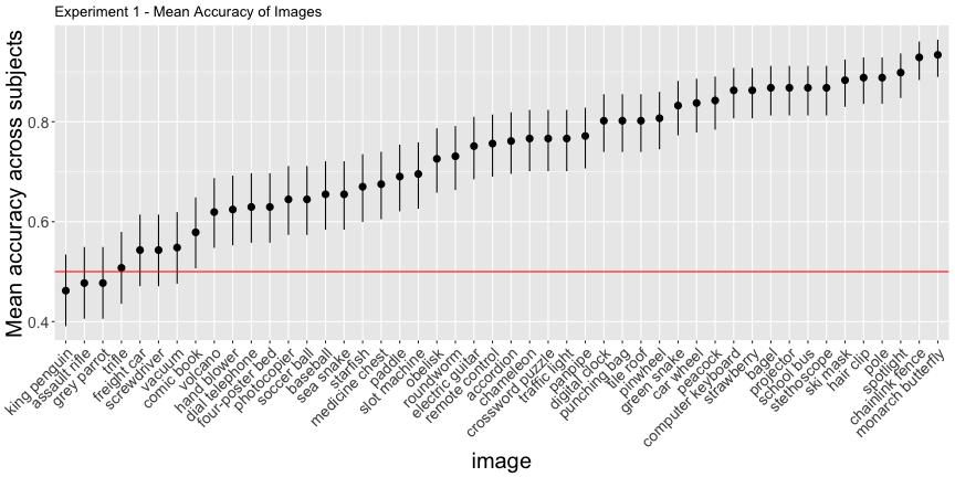
g.e1_subject <- plot_subject(e1_subject, "1")
g.e1_subject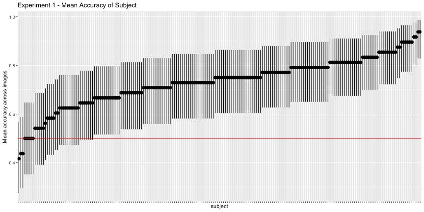
So far so good, although if we use the binomial confidence intervals rather than just the mean response rate – what I’ll call corrected accuracies – we get a more valid description of above-chance accuracy
e1_accs <- adjusted_accuracy(e1_image, e1_subject)Only 85.4% of images were categorized above chance, and 81.2% of subjects did, as opposed to the reported 94% and 98%, respectively.
Experiment 2 - 1st vs 2nd best labels
Of course, not all foil labels are created equal, so a more conservative test for human/machine overlap is to compare the highest and second highest labels predicted by the machine.
e2_summary <- summarize_data(expt_2)
e2_image <- e2_summary$image
e2_subject <- e2_summary$subject
g.e2_img <- plot_image(e2_image, "2")
g.e2_img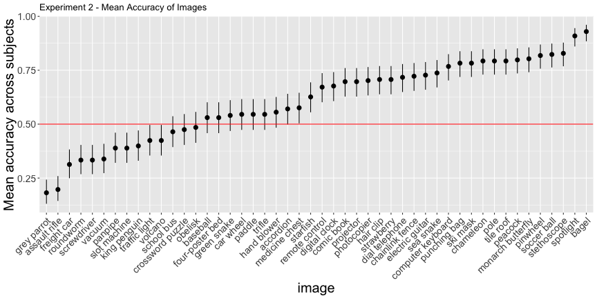
g.e2_subject <- plot_subject(e2_subject, "2")
g.e2_subject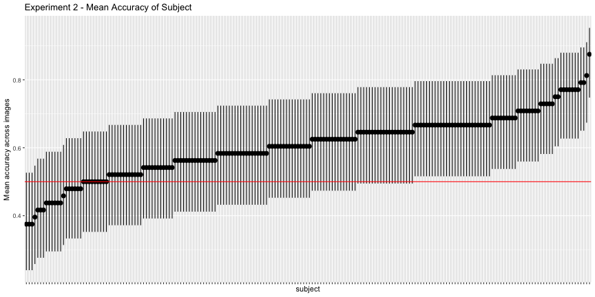
This looks much worse, and the corrected accuracies reflect that
e2_accs <- adjusted_accuracy(e2_image, e2_subject)

total_acc <- nrow(expt_2[expt_2$correct== TRUE,])/nrow(expt_2)
total_acc <- round(total_acc, 3) * 100
Only 54.2% of images and 31.3% of subjects classified above chance, as opposed to the reported 71% and 91%, respectively.
Collapsing across all images and subjects, only 60.6% of responses agreed with the top category of the CNN.
We can see the accuracy-inflating strength of having bad foils by comparing experiment 1 vs 2. Images whose classifications remained high in experiment 2 are robust to their next-best label, while those that are significantly worse in experiment 2 are vulnerable.
e12_images <- left_join(e1_image, e2_image, by="image")## Warning: Column `image` joining factors with different levels, coercing to
## character vectore12_images$image <- ordered(e12_images$image, levels=e12_images$image[order(e12_images$meancx.x)])ggplot(e12_images, aes(x=image, ymin=cilo.x, ymax=cihi.x, y=meancx.x))+
geom_pointrange()+
geom_pointrange(aes(ymin=cilo.y, ymax=cihi.y, y=meancx.y),color="red")+
geom_hline(yintercept = 0.5, color="red")+
labs(title="Experiment 1 vs Experiment 2 - Mean Accuracy of Images",
y="Mean accuracy across subjects")+
theme(axis.text.x = element_text(angle=45, hjust=1))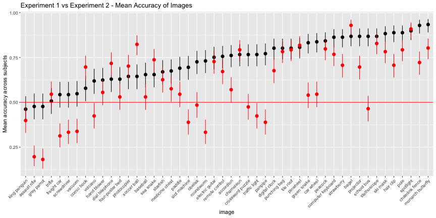
Experiments 3a and 3b
Experiments 3a and 3b presented all possible labels instead of two. 3a was the “machine theory of mind” task, and 3b asked subjects to rate what they thought the images were. First, the overall summaries of 3a
e3a_summary <- summarize_data(expt_3a)
e3a_image <- e3a_summary$image
e3a_subject <- e3a_summary$subject


e3b_summary <- summarize_data(expt_3b)
e3b_image <- e3b_summary$image
e3b_subject <- e3b_summary$subject
g.e3a_image <- plot_image(e3a_image, "3a")
g.e3a_image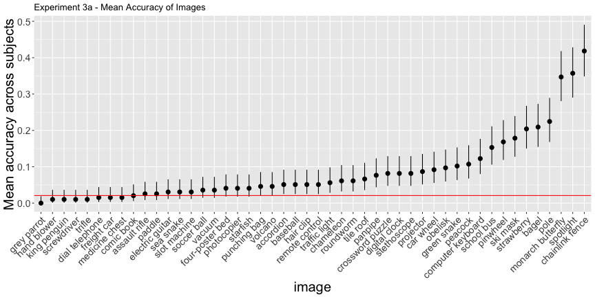
g.e3a_sub <- plot_subject(e3a_subject, "3a")
g.e3a_sub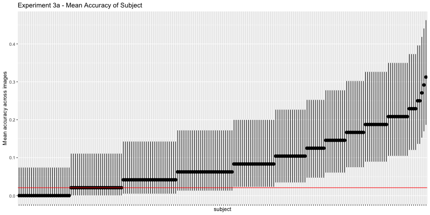
e3a_acc <- adjusted_accuracy(e3a_image, e3a_subject, level=1/48)Again, only 60.4% of images and 47.4% of subjects were above chance accuracy of 1/48, as opposed to the reported 79% and 88%, respectively. Experiment 3b has qualitatively the same results, but their interpretation doesn’t necessarily follow from the data:
These results suggest that the humans’ability to decipher adversarial images doesn’t depend on the peculiarities of our machine-theory-of-mind task, and that human performance reflects a more general agreement with machine (mis)classification.
There are actually two degenerate interpretations here: either human performance is the same as machine performance, or the subjects were just rating what they thought the images were in all tasks. No further differentiating experiments were done to tease these interpretations apart, so this point is a wash.
Further, if one looks at the most accurately categorized images…
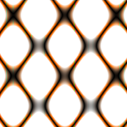
Chainlink fence

Spotlight
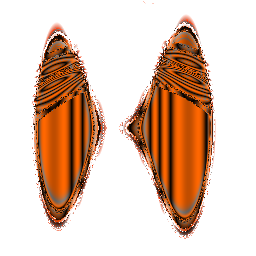
Monarch Butterfly
… we can easily see why they were. Remember the argument here is that these are supposedly adversarial images that fool a classifier. A finding that humans and image classification algorithms similarly categorize things that really do look like those categories is unremarkable.
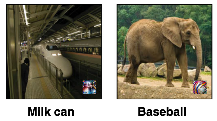
Experiment 4 - Static images
Experiment 4 uses “static” images (from the same source paper), but also changes the task in a meaningful way. Rather than asking what category an image was, the subject is presented with the category and a set of representative images and asked “which image has this category?”
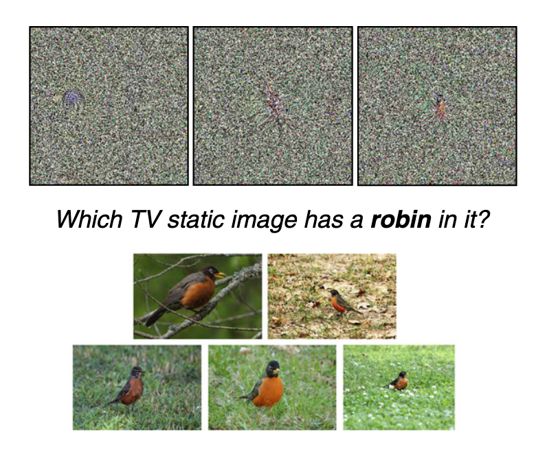
This experiment only has 8 images in the set of static images, and each is presented in every trial. The authors note that
upon very close inspection, you may notice a small, often central,‘object’ within each image.
and they are actually quite pronounced. Even if the central “objects” don’t look recognizably like the categorized object, they are distinguishable that subjects should be able to recognize them between trials. Since the subjects are asked to choose one category for each of the images, it seems possible for them to use that information to exclude images from later trials. In other words, the trials are not independent. This is reflected in the positive slope of accuracy over trial number
e4_sum <- summarize_e4(expt_4)
e4_image <- e4_sum$image
e4_subject <- e4_sum$subject
e4_trial <- e4_sum$trial

e4_accs <- adjusted_accuracy(e4_image, e4_subject, level=1/8)ggplot(e4_trial, aes(x=trialNum, y=meancx))+
geom_pointrange(aes(ymin=cilo, ymax=cihi))+
geom_smooth(method="lm")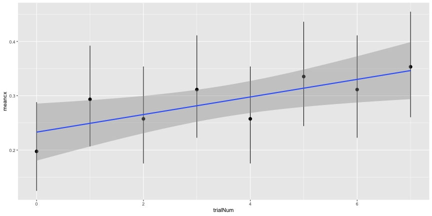
e4_lm <- lm(meancx~trialNum, data=e4_trial)
summary(e4_lm)
##
## Call:
## lm(formula = meancx ~ trialNum, data = e4_trial)
##
## Residuals:
## Min 1Q Median 3Q Max
## -0.040277 -0.022918 -0.000463 0.023489 0.044197
##
## Coefficients:
## Estimate Std. Error t value Pr(>|t|)
## (Intercept) 0.233034 0.021472 10.853 3.63e-05 ***
## trialNum 0.016182 0.005133 3.153 0.0197 *
## ---
## Signif. codes: 0 '***' 0.001 '**' 0.01 '*' 0.05 '.' 0.1 ' ' 1
##
## Residual standard error: 0.03326 on 6 degrees of freedom
## Multiple R-squared: 0.6236, Adjusted R-squared: 0.5608
## F-statistic: 9.939 on 1 and 6 DF, p-value: 0.01975g.e4_image <- plot_image(e4_image, "4")
g.e4_image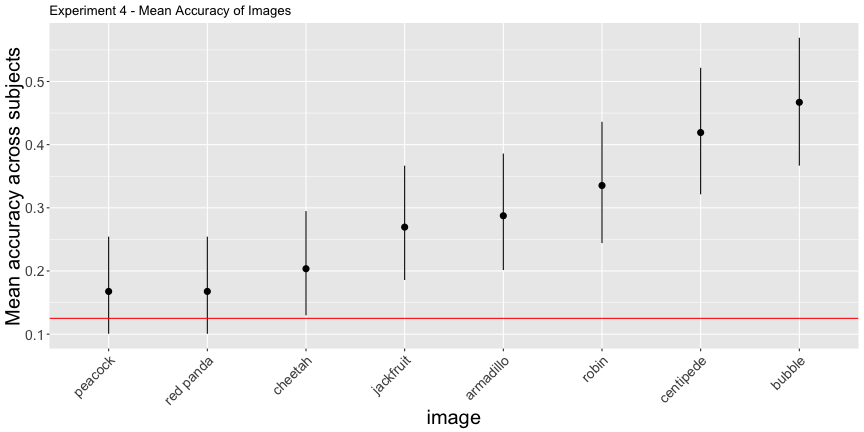
g.e4_subject <- plot_subject(e4_subject, "4")
g.e4_subject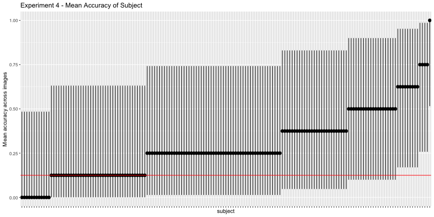
Again, the corrected accuracies are much lower than they report, accounting for uncertainty, only 75% of images and 8.4% of subjects had accuracies above chance, rather than the reported 100% and 81%, respectively. This is exceptionally troubling for their interpretation of their results, as it is subject accuracy that matters, not image accuracy.
Experiment 5 - Digit classification
In this experiment, perturbed MNIST digits are given, and the subjects are told they were miscategorized – ie. choose the mistaken digit NOT the one that it looks like.
As a first pass, things look ok…
e5_sum <- summarize_e5(expt_5)
e5_image <- e5_sum$image
e5_subject <- e5_sum$subject
e5_image$image <- e5_image$target

e5_accs <- adjusted_accuracy(e5_image, e5_subject, level=1/9)
g.e5_image <- plot_image(e5_image, "5")
g.e5_image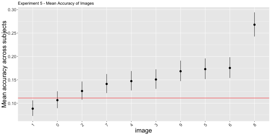
But something is off with the confusion matrix
expt_5$response <- as.factor(expt_5$response)
expt_5$target <- as.factor(expt_5$target)
cm5 <- caret::confusionMatrix(expt_5$response, expt_5$target)
cm5 <- reshape2::melt(cm5$table)ggplot(cm5, aes(x=as.factor(Reference), y=as.factor(Prediction), fill=value))+
geom_tile()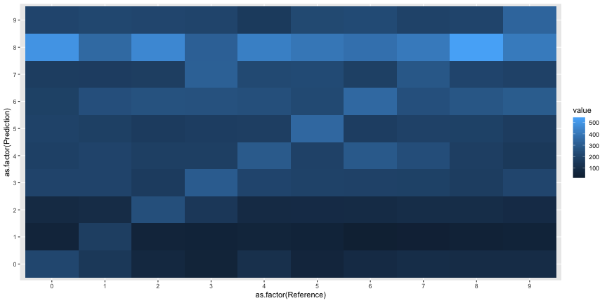
It looks like everyone just said everything was an 8. In the plot below, the rate of “8” responses is colored in red.
ggplot(e5_image, aes(x=target, ymin=cilo, ymax=cihi, y=meancx))+
  geom_pointrange()+
  geom_pointrange(aes(ymin=cilo8, ymax=cihi8, y=meaneight), color="red")+
  geom_hline(yintercept = 1/9, color="red")+
  labs(title="Experiment 5 - black = mean correct responses, red = mean 8 responses")+
  theme(axis.text.x = element_text(angle=45, hjust=1))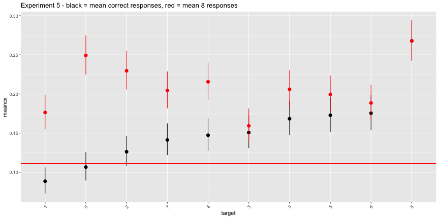
The interpretation of this experiment given in the paper is straightforwardly inaccurate. Most subjects did not agree with the machine classification, they just classified everything as an 8. The “above chance accuracy” of the target labels was only due to the very low rates of other digit responses.
This is reflected in the subject accuracy, where only 15.1% of subjects had accuracies significantly better than chance.
g.e5_subject <- plot_subject(e5_subject, "5")
g.e5_subject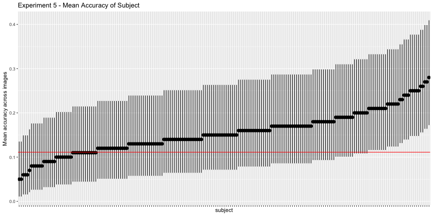
Experiment 6
e6_sum <- summarize_6(expt_6)
e6_image <- e6_sum$image
e6_subject <- e6_sum$subject
e6_image$image <- e6_image$target

e6_accs <- adjusted_accuracy(e6_image, e6_subject, level=0.5)
g.e6_image <- plot_image(e6_image, "6")
g.e6_image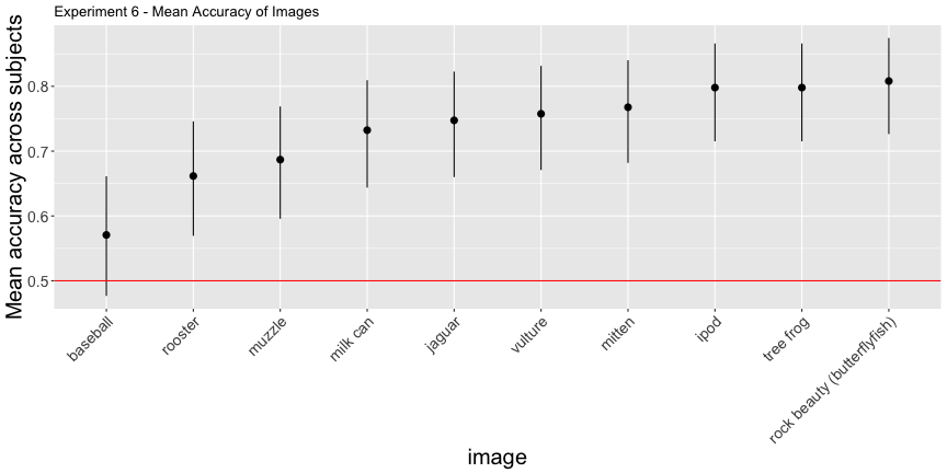
g.e6_subject <- plot_subject(e6_subject, "6")
g.e6_subject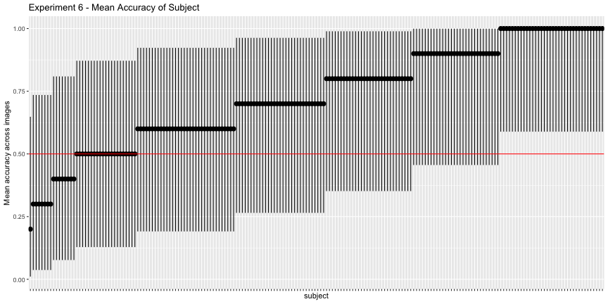
These images have surprisingly high accuracy! At last! This one seems solid.
However, the image perturbation introduces small images that look exactly like the target category into the images. Some examples:
The “rock beauty” fish with the highest accuracy: 
and the milk jug 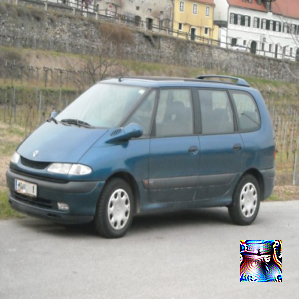
This is especially problematic since the task was to choose one of two labels – as was the case in experiment 1 as compared to 2, even when the primary label isn’t immediately obvious, if the foil label is significantly worse the categorization becomes trivial.
Experiment 7
e7_sum <- summarize_7(expt_7)
e7_image <- e7_sum$image
e7_subject <- e7_sum$subject
e7_image$image <- e7_image$imageName
e7_accs <- adjusted_accuracy(e7_image, e7_subject, 0.5)

e7_total <- round(sum(expt_7$correct)/nrow(expt_7), 3)*100
g.e7_image <- plot_image(e7_image, "7")
g.e7_image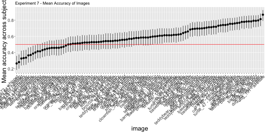
g.e7_subject <- plot_subject(e7_subject, "7")
g.e7_subject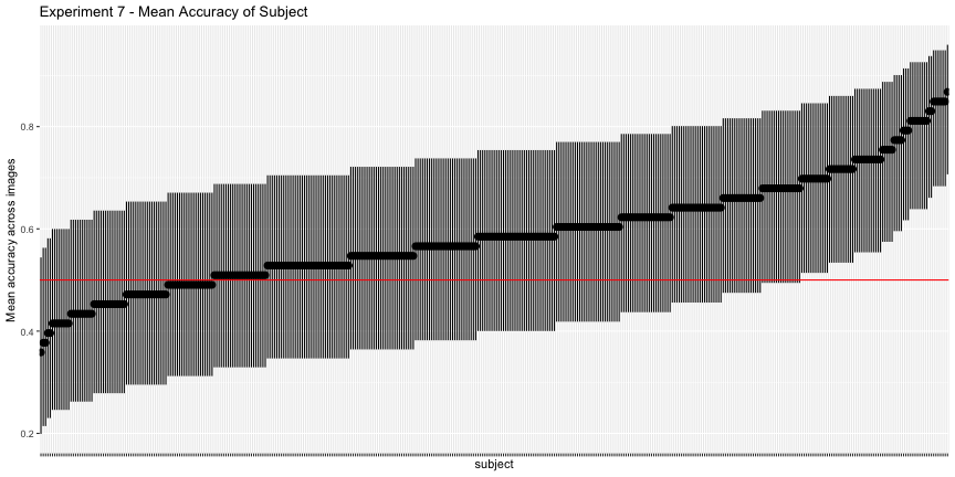
Again, only 44.3% of images and 16.3% of subjects had accuracy significantly above chance, as opposed to the reported 78% of images and 83% of subjects. Overall, across all images and subjects, the total accuracy was 58.9%.
The image synthesis technique is tuned to minimize perceptual perturbations, but does impart a recognizable texture to the objects in the image. This was especially problematic in examples where the original image and the target class were semantically related, or had a similar texture, for example
A dog_191, whose adversarial target was “airedale”
In others, the texture was so obvious that it is no longer visually undetectable.
 Dog 63, whose adversarial target was “indian cobra.”
e7_acc_total <- sum(expt_7$correct)/nrow(expt_7)Overall summary
e4_image$meanrt <- NA
e5_image$meanrt <- NA
e6_image$meanrt <- NA
e7_image$meanrt <- NA

e5_sub <- e5_image[,-c(5,6,7,8)]
e3a_accs <- adjusted_accuracy(e3a_image, e3a_subject, level=1/48)
e3b_accs <- adjusted_accuracy(e3b_image, e3b_subject,level=1/48)
all_images <- bind_rows("expt_1"=e1_accs,
                    "expt_2"=e2_accs,
                    "expt_3a"=e3a_accs,
                    "expt_3b"=e3b_accs,
                    "expt_4"=e4_accs,
                    "expt_5"=e5_accs,
                    "expt_6"=e6_accs,
                    "expt_7"=e7_accs,
                    .id="expt")

all_images$reported_img <-     c(94, 71, 79, 81, 100, 73, 100, 78)
all_images$reported_subject <- c(98, 91, 88, 90, 81,  89, 87,  83)

all_im_melt <- reshape2::melt(all_images, measure.vars=c("image", "subject", "reported_img", "reported_subject"))

all_im_melt$type <- "image"
all_im_melt[all_im_melt$variable %in% c("subject", "reported_subject"),]$type <- "subject"

all_im_melt$which <- "adjusted"
all_im_melt[all_im_melt$variable %in% c("reported_subject", "reported_img"),]$which <- "reported"

all_im_melt$expt <- ordered(all_im_melt$expt, levels=experiment_names)
all_im_melt$type <- ordered(all_im_melt$type, levels=c("image", "subject"))
all_im_melt$which <- ordered(all_im_melt$which, levels=c("reported", "adjusted"))

all_im_melt$which_type <- paste(all_im_melt$type, all_im_melt$which)
all_im_melt$which_type <- ordered(all_im_melt$which_type, levels=c("image reported", "subject reported", "image adjusted", "subject adjusted"))ggplot(all_im_melt, aes(x=expt, y=value,
fill=which_type))+
geom_col(position="dodge")+
scale_fill_brewer(palette="Paired")+
theme(axis.text.x=element_text(angle=45,hjust=1))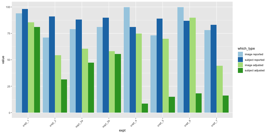
library(tidyverse)
library(lme4)
library(rio)
library(binom)
library(here)
library(caret)
I’ve put the data in a directory in my website structure, “/assets/data/adv”. We’ll load them all into variable names expt_1, expt_2, etc. and do some cleanup.
# list experiment data files
experiment_dirs <- list.dirs(here('assets', 'data', 'adv'), full.names=FALSE, recursive=FALSE)

# name each dataset according to its number
experiment_names <- c("expt_1", "expt_2", "expt_3a", "expt_3b", "expt_4", "expt_5", "expt_6", "expt_7")

# list the datafiles
data_files <- c()
for (i in seq(length(experiment_dirs))){
  data_files[i] <- list.files(here('assets', 'data', 'adv', experiment_dirs[i], "data"), full.names = TRUE)[1]
}

# load experiments
for (i in seq(length(data_files))){
  assign(experiment_names[i],
         as.tbl(import_list(data_files[i])$Data))
}

##########################
## clean data

# rename columns
names(expt_1)[c(1, 9, 10, 11)] <- c("subject", "correct", "rt_pass", "complete")
names(expt_2)[c(1, 9, 10, 11)] <- c("subject", "correct", "rt_pass", "complete")
names(expt_3a)[c(1, 6, 7, 8)] <- c("subject", "correct", "rt_pass", "complete")
names(expt_3b)[c(1, 6, 7, 8)] <- c("subject", "correct", "rt_pass", "complete")
names(expt_4)[c(1,6,7,8,9)] <- c("subject", "correct", "rt_pass", "rt_allpass", "complete")
names(expt_5)[c(1,7,8,9)] <- c("subject", "correct", "rt_pass",  "complete")
names(expt_6)[c(1,10,11,12)] <- c("subject", "correct", "rt_pass", "complete")
names(expt_7)[c(1,10,11,12)] <- c("subject", "correct", "rt_pass", "complete")

# retype columns
for (expt_name in experiment_names){
  # use get to refer to the object with its character name not its symbol name
  xpt <- get(expt_name)

    # subset incomplete subjects
  xpt <- xpt[xpt$complete == TRUE,]
  if ("rt_allpass" %in% names(xpt)){
    xpt <- xpt[xpt$rt_allpass==TRUE,]
  }

  # first columns present in all dfs
  xpt <- xpt %>% mutate(
    subject = as.factor(subject),
    correct = as.logical(correct),
    rt_pass = as.logical(rt_pass),
    complete = as.logical(complete)
  )

  # then specifics
  if ("image" %in% names(xpt)){
    xpt$image <- as.factor(xpt$image)
  }

  if ("response" %in% names(xpt)){
    xpt$response <- as.factor(xpt$response)
  }


  # assign back to name

  assign(expt_name,
         xpt)
}
Summarizing Functions
Since so much of the data has the same structure, we’ll write functions to summarize the image responses by image and subject. They’ll return
n_trials- the number of trials per groupn_correct- the number of “correct,” or matching the categorization of the CNN, trialsmeancx- the proportion of correct answers per groupcilo,cihi- the 95% confidence interval around the mean correct.
summarize_data <- function(data){

  summary_image <- data %>% group_by(image) %>%
  summarize(n_trials = length(correct),
            n_correct = sum(correct),
            meancx = n_correct/n_trials,
            meanrt = mean(rt),
            sdrt = sd(rt),
            cilo = binom.confint(sum(correct),length(correct),
                                  conf.level=0.95,method="exact")[[5]],
            cihi = binom.confint(sum(correct),length(correct),
                                  conf.level=0.95,method="exact")[[6]])

  summary_image$image <- ordered(summary_image$image,
                              levels=summary_image$image[order(summary_image$meancx)])

  summary_subject <- data %>% group_by(subject) %>%
    summarize(n_trials = length(correct),
              n_correct = sum(correct),
              meancx = n_correct/n_trials,
              meanrt = mean(rt),
              sdrt = sd(rt),
              cilo = binom.confint(sum(correct),length(correct),
                                   conf.level=0.95,method="exact")[[5]],
              cihi = binom.confint(sum(correct),length(correct),
                                   conf.level=0.95,method="exact")[[6]])

  summary_subject$subject <- ordered(summary_subject$subject,
                                     levels=summary_subject$subject[order(summary_subject$meancx)])

  return(list("image" = summary_image,
              "subject" = summary_subject))

}

summarize_e4 <- function(e4){
  names(e4)[c(1,6,7,8,9)] <- c("subject", "correct", "rt_pass", "rt_allpass", "complete")
  e4 <- e4[(e4$complete == TRUE) & (e4$rt_allpass == TRUE),]
  e4$subject <- as.factor(e4$subject)
  e4$target <- as.factor(e4$target)
  e4$response <- as.factor(e4$response)
  e4$trialNum <- as.integer(e4$trialNum)

  e4_image <- e4 %>% group_by(target) %>%
    summarize(n_trials = length(correct),
              n_correct = sum(correct),
              meancx = n_correct/n_trials,
              cilo = binom.confint(sum(correct),length(correct),
                                   conf.level=0.99,method="exact",
                                   alternative="greater")[[5]],
              cihi = binom.confint(sum(correct),length(correct),
                                   conf.level=0.99,method="exact",
                                   alternative="greater")[[6]])

  e4_subject <- e4 %>% group_by(subject) %>%
    summarize(n_trials = length(correct),
              n_correct = sum(correct),
              meancx = n_correct/n_trials,
              cilo = binom.confint(sum(correct),length(correct),
                                   conf.level=0.99,method="exact",
                                   alternative="greater")[[5]],
              cihi = binom.confint(sum(correct),length(correct),
                                   conf.level=0.99,method="exact",
                                   alternative="greater")[[6]])

  e4_trial <- e4 %>% group_by(trialNum) %>%
    summarize(n_trials = length(correct),
              n_correct = sum(correct),
              meancx = n_correct/n_trials,
              cilo = binom.confint(sum(correct),length(correct),
                                   conf.level=0.99,method="exact",
                                   alternative="greater")[[5]],
              cihi = binom.confint(sum(correct),length(correct),
                                   conf.level=0.99,method="exact",
                                   alternative="greater")[[6]])

  e4_image$target <- ordered(e4_image$target, levels=e4_image$target[order(e4_image$meancx)])
  e4_image$image <- e4_image$target
  e4_subject$subject <- ordered(e4_subject$subject, levels=e4_subject$subject[order(e4_subject$meancx)])
  return(list("image"=e4_image,
              "subject"=e4_subject,
              "trial"=e4_trial))
}

summarize_e5 <- function(e5){

e5_image <- e5 %>% group_by(target) %>%
  summarize(n_trials = length(correct),
            n_correct = sum(correct),
            meancx = n_correct/n_trials,
            n_eight = sum(response == "8"),
            meaneight = n_eight/n_trials,
            cilo8 = binom.confint(n_eight,length(correct),
                                  conf.level=0.99,method="exact",
                                  alternative="greater")[[5]],
            cihi8 = binom.confint(n_eight,length(correct),
                                  conf.level=0.99,method="exact",
                                  alternative="greater")[[6]],
            cilo = binom.confint(sum(correct),length(correct),
                                 conf.level=0.99,method="exact",
                                 alternative="greater")[[5]],
            cihi = binom.confint(sum(correct),length(correct),
                                 conf.level=0.99,method="exact",
                                 alternative="greater")[[6]])


e5_subject <- e5 %>% group_by(subject) %>%
  summarize(n_trials = length(correct),
            n_correct = sum(correct),
            meancx = n_correct/n_trials,
            cilo = binom.confint(sum(correct),length(correct),
                                 conf.level=0.99,method="exact",
                                 alternative="greater")[[5]],
            cihi = binom.confint(sum(correct),length(correct),
                                 conf.level=0.99,method="exact",
                                 alternative="greater")[[6]])


e5_image$target <- ordered(e5_image$target, levels=e5_image$target[order(e5_image$meancx)])
e5_subject$subject <- ordered(e5_subject$subject, levels=e5_subject$subject[order(e5_subject$meancx)])
return(list("image"=e5_image,
            "subject"=e5_subject))
}

summarize_6 <- function(e6){

e6_image <- e6 %>% group_by(target) %>%
  summarize(n_trials = length(correct),
            n_correct = sum(correct),
            meancx = n_correct/n_trials,
            cilo = binom.confint(sum(correct),length(correct),
                                 conf.level=0.99,method="exact",
                                 alternative="greater")[[5]],
            cihi = binom.confint(sum(correct),length(correct),
                                 conf.level=0.99,method="exact",
                                 alternative="greater")[[6]])


e6_subject <- e6 %>% group_by(subject) %>%
  summarize(n_trials = length(correct),
            n_correct = sum(correct),
            meancx = n_correct/n_trials,
            cilo = binom.confint(sum(correct),length(correct),
                                 conf.level=0.99,method="exact",
                                 alternative="greater")[[5]],
            cihi = binom.confint(sum(correct),length(correct),
                                 conf.level=0.99,method="exact",
                                 alternative="greater")[[6]])


e6_image$target <- ordered(e6_image$target, levels=e6_image$target[order(e6_image$meancx)])
e6_subject$subject <- ordered(e6_subject$subject, levels=e6_subject$subject[order(e6_subject$meancx)])
return(list("image"=e6_image,
            "subject"=e6_subject))

}


summarize_7 <- function(e7){

e7_image <- e7 %>% group_by(imageName) %>%
  summarize(n_trials = length(correct),
            n_correct = sum(correct),
            meancx = n_correct/n_trials,
            target = target[1],
            cilo = binom.confint(sum(correct),length(correct),
                                 conf.level=0.99,method="exact",
                                 alternative="greater")[[5]],
            cihi = binom.confint(sum(correct),length(correct),
                                 conf.level=0.99,method="exact",
                                 alternative="greater")[[6]])


e7_subject <- e7 %>% group_by(subject) %>%
  summarize(n_trials = length(correct),
            n_correct = sum(correct),
            meancx = n_correct/n_trials,
            cilo = binom.confint(sum(correct),length(correct),
                                 conf.level=0.99,method="exact",
                                 alternative="greater")[[5]],
            cihi = binom.confint(sum(correct),length(correct),
                                 conf.level=0.99,method="exact",
                                 alternative="greater")[[6]])


e7_image$imageName <- ordered(e7_image$imageName, levels=e7_image$imageName[order(e7_image$meancx)])
e7_subject$subject <- ordered(e7_subject$subject, levels=e7_subject$subject[order(e7_subject$meancx)])
return(list("image"=e7_image,
            "subject"=e7_subject))

}

# and some convenience functions to make our basic plots
plot_image <- function(ex_image, ex_num){
  if (ex_num %in% c("3a", "3b")){
    y_height = 1/48
  } else if (ex_num == "4"){
    y_height = 1/8
  } else if (ex_num == "5"){
    y_height = 1/9
  } else {
    y_height = 0.5
  }

  if (ex_num == "7"){
    ex_image$image <- paste(ex_image$image, ex_image$target, sep=" - ")
    ex_image$image <- ordered(ex_image$image, levels=ex_image$image[order(ex_image$meancx)])
  }

  g.image <- ggplot(ex_image, aes(x=image, y=meancx, ymin=cilo, ymax=cihi))+
  geom_pointrange()+
  geom_hline(yintercept = y_height, color="red")+
  labs(title=paste("Experiment", ex_num, "- Mean Accuracy of Images"),
       y="Mean accuracy across subjects")+
  theme(axis.text = element_text(size=unit(14,"pt")),
        axis.title = element_text(size=unit(20,"pt")),
    axis.text.x = element_text(angle=45, hjust=1))

  return(g.image)
}

plot_subject <- function(ex_subject, ex_num){

  if (ex_num %in% c("3a", "3b")){
    y_height = 1/48
  } else if (ex_num == "4"){
    y_height=1/8
  } else if (ex_num == "5"){
    y_height=1/9
  } else {
    y_height = 0.5
  }

  g.subject <- ggplot(ex_subject, aes(x=subject, y=meancx, ymin=cilo, ymax=cihi))+
  geom_pointrange()+
  geom_hline(yintercept = y_height, color="red")+
  labs(title=paste("Experiment", ex_num, "- Mean Accuracy of Subject"),
       y="Mean accuracy across images")+
  theme(axis.text.x = element_blank())

  return(g.subject)
}

# and to compute subject and image accuracies using confidence intervals instead of means
adjusted_accuracy <- function(ex_image, ex_subject, level=0.5){
  ex_img_accuracy <- nrow(ex_image[ex_image$cilo>level,])/nrow(ex_image)
  ex_subject_accuracy <- nrow(ex_subject[ex_subject$cilo>level,])/nrow(ex_subject)

# round for inclusion in the text
ex_img_accuracy <- round(ex_img_accuracy, 3)*100
ex_subject_accuracy <- round(ex_subject_accuracy,3)*100

  return(list(image = ex_img_accuracy,
              subject = ex_subject_accuracy))
}
Experiment 1
The first image uses images from Nguyen A, et al 2014, which were generated using a “compositional pattern-producing network” that
can produce images that both humans and DNNs can recognize.
Importantly though,
These images were produced on PicBreeder.org, a site where users serve as the fitness function in an evolutionary algorithm by selecting images they like, which become the parents of the next generation.
So using these images may make the results particularly difficult to interpret, as it’s not clear how aesthetic preference interacts with the preference for recognizable objects. It could be the case that people pick images to preserve in the image generation process that look like real objects, so they aren’t “adversarial” images, strictly speaking. Indeed, the authors of the image-generation paper note
the generated images do often contain some features of the target class
so a human classifying an image as the same class as a machine might be unsurprising for these images. Since some of the images do indeed resemble the ‘target’ classes, those images are unsuitable for assessing the degree to which the human visual system makes the same ‘errors’ as machine vision.
The subjects in this task saw one of 48 “fooling images,” and were presented with the “correct” label and a randomly selected label from the other 47 images. The primary result the report for this experiment is that
98% of observers chose the machine’s label at above-chance rates. […] Additionally, 94% of the images showed above-chance human-machine agreement
Reanalyzing by image and subject, however…
# summarize the data and expand list to new
sum_1 <- summarize_data(expt_1)
e1_image <- sum_1$image
e1_subject <- sum_1$subject
g.e1_image <- plot_image(e1_image, "1")
g.e1_image
g.e1_subject <- plot_subject(e1_subject, "1")
g.e1_subject
So far so good, although if we use the binomial confidence intervals rather than just the mean response rate – what I’ll call corrected accuracies – we get a more valid description of above-chance accuracy
e1_accs <- adjusted_accuracy(e1_image, e1_subject)Only 85.4% of images were categorized above chance, and 81.2% of subjects did, as opposed to the reported 94% and 98%, respectively.
Experiment 2 - 1st vs 2nd best labels
Of course, not all foil labels are created equal, so a more conservative test for human/machine overlap is to compare the highest and second highest labels predicted by the machine.
e2_summary <- summarize_data(expt_2)
e2_image <- e2_summary$image
e2_subject <- e2_summary$subject
g.e2_img <- plot_image(e2_image, "2")
g.e2_img
g.e2_subject <- plot_subject(e2_subject, "2")
g.e2_subject
This looks much worse, and the corrected accuracies reflect that
e2_accs <- adjusted_accuracy(e2_image, e2_subject)

total_acc <- nrow(expt_2[expt_2$correct== TRUE,])/nrow(expt_2)
total_acc <- round(total_acc, 3) * 100
Only 54.2% of images and 31.3% of subjects classified above chance, as opposed to the reported 71% and 91%, respectively.
Collapsing across all images and subjects, only 60.6% of responses agreed with the top category of the CNN.
We can see the accuracy-inflating strength of having bad foils by comparing experiment 1 vs 2. Images whose classifications remained high in experiment 2 are robust to their next-best label, while those that are significantly worse in experiment 2 are vulnerable.
e12_images <- left_join(e1_image, e2_image, by="image")## Warning: Column `image` joining factors with different levels, coercing to
## character vectore12_images$image <- ordered(e12_images$image, levels=e12_images$image[order(e12_images$meancx.x)])ggplot(e12_images, aes(x=image, ymin=cilo.x, ymax=cihi.x, y=meancx.x))+
geom_pointrange()+
geom_pointrange(aes(ymin=cilo.y, ymax=cihi.y, y=meancx.y),color="red")+
geom_hline(yintercept = 0.5, color="red")+
labs(title="Experiment 1 vs Experiment 2 - Mean Accuracy of Images",
y="Mean accuracy across subjects")+
theme(axis.text.x = element_text(angle=45, hjust=1))
Experiments 3a and 3b
Experiments 3a and 3b presented all possible labels instead of two. 3a was the “machine theory of mind” task, and 3b asked subjects to rate what they thought the images were. First, the overall summaries of 3a
e3a_summary <- summarize_data(expt_3a)
e3a_image <- e3a_summary$image
e3a_subject <- e3a_summary$subject


e3b_summary <- summarize_data(expt_3b)
e3b_image <- e3b_summary$image
e3b_subject <- e3b_summary$subject
g.e3a_image <- plot_image(e3a_image, "3a")
g.e3a_image
g.e3a_sub <- plot_subject(e3a_subject, "3a")
g.e3a_sub
e3a_acc <- adjusted_accuracy(e3a_image, e3a_subject, level=1/48)Again, only 60.4% of images and 47.4% of subjects were above chance accuracy of 1/48, as opposed to the reported 79% and 88%, respectively. Experiment 3b has qualitatively the same results, but their interpretation doesn’t necessarily follow from the data:
These results suggest that the humans’ability to decipher adversarial images doesn’t depend on the peculiarities of our machine-theory-of-mind task, and that human performance reflects a more general agreement with machine (mis)classification.
There are actually two degenerate interpretations here: either human performance is the same as machine performance, or the subjects were just rating what they thought the images were in all tasks. No further differentiating experiments were done to tease these interpretations apart, so this point is a wash.
Further, if one looks at the most accurately categorized images…
Chainlink fence
Spotlight
Monarch Butterfly
… we can easily see why they were. Remember the argument here is that these are supposedly adversarial images that fool a classifier. A finding that humans and image classification algorithms similarly categorize things that really do look like those categories is unremarkable.
Experiment 4 - Static images
Experiment 4 uses “static” images (from the same source paper), but also changes the task in a meaningful way. Rather than asking what category an image was, the subject is presented with the category and a set of representative images and asked “which image has this category?”
This experiment only has 8 images in the set of static images, and each is presented in every trial. The authors note that
upon very close inspection, you may notice a small, often central,‘object’ within each image.
and they are actually quite pronounced. Even if the central “objects” don’t look recognizably like the categorized object, they are distinguishable that subjects should be able to recognize them between trials. Since the subjects are asked to choose one category for each of the images, it seems possible for them to use that information to exclude images from later trials. In other words, the trials are not independent. This is reflected in the positive slope of accuracy over trial number
e4_sum <- summarize_e4(expt_4)
e4_image <- e4_sum$image
e4_subject <- e4_sum$subject
e4_trial <- e4_sum$trial

e4_accs <- adjusted_accuracy(e4_image, e4_subject, level=1/8)ggplot(e4_trial, aes(x=trialNum, y=meancx))+
geom_pointrange(aes(ymin=cilo, ymax=cihi))+
geom_smooth(method="lm")
e4_lm <- lm(meancx~trialNum, data=e4_trial)
summary(e4_lm)
##
## Call:
## lm(formula = meancx ~ trialNum, data = e4_trial)
##
## Residuals:
## Min 1Q Median 3Q Max
## -0.040277 -0.022918 -0.000463 0.023489 0.044197
##
## Coefficients:
## Estimate Std. Error t value Pr(>|t|)
## (Intercept) 0.233034 0.021472 10.853 3.63e-05 ***
## trialNum 0.016182 0.005133 3.153 0.0197 *
## ---
## Signif. codes: 0 '***' 0.001 '**' 0.01 '*' 0.05 '.' 0.1 ' ' 1
##
## Residual standard error: 0.03326 on 6 degrees of freedom
## Multiple R-squared: 0.6236, Adjusted R-squared: 0.5608
## F-statistic: 9.939 on 1 and 6 DF, p-value: 0.01975g.e4_image <- plot_image(e4_image, "4")
g.e4_image
g.e4_subject <- plot_subject(e4_subject, "4")
g.e4_subject
Again, the corrected accuracies are much lower than they report, accounting for uncertainty, only 75% of images and 8.4% of subjects had accuracies above chance, rather than the reported 100% and 81%, respectively. This is exceptionally troubling for their interpretation of their results, as it is subject accuracy that matters, not image accuracy.
Experiment 5 - Digit classification
In this experiment, perturbed MNIST digits are given, and the subjects are told they were miscategorized – ie. choose the mistaken digit NOT the one that it looks like.
As a first pass, things look ok…
e5_sum <- summarize_e5(expt_5)
e5_image <- e5_sum$image
e5_subject <- e5_sum$subject
e5_image$image <- e5_image$target

e5_accs <- adjusted_accuracy(e5_image, e5_subject, level=1/9)
g.e5_image <- plot_image(e5_image, "5")
g.e5_image
But something is off with the confusion matrix
expt_5$response <- as.factor(expt_5$response)
expt_5$target <- as.factor(expt_5$target)
cm5 <- caret::confusionMatrix(expt_5$response, expt_5$target)
cm5 <- reshape2::melt(cm5$table)ggplot(cm5, aes(x=as.factor(Reference), y=as.factor(Prediction), fill=value))+
geom_tile()
It looks like everyone just said everything was an 8. In the plot below, the rate of “8” responses is colored in red.
ggplot(e5_image, aes(x=target, ymin=cilo, ymax=cihi, y=meancx))+
  geom_pointrange()+
  geom_pointrange(aes(ymin=cilo8, ymax=cihi8, y=meaneight), color="red")+
  geom_hline(yintercept = 1/9, color="red")+
  labs(title="Experiment 5 - black = mean correct responses, red = mean 8 responses")+
  theme(axis.text.x = element_text(angle=45, hjust=1))
The interpretation of this experiment given in the paper is straightforwardly inaccurate. Most subjects did not agree with the machine classification, they just classified everything as an 8. The “above chance accuracy” of the target labels was only due to the very low rates of other digit responses.
This is reflected in the subject accuracy, where only 15.1% of subjects had accuracies significantly better than chance.
g.e5_subject <- plot_subject(e5_subject, "5")
g.e5_subject
Experiment 6
e6_sum <- summarize_6(expt_6)
e6_image <- e6_sum$image
e6_subject <- e6_sum$subject
e6_image$image <- e6_image$target

e6_accs <- adjusted_accuracy(e6_image, e6_subject, level=0.5)
g.e6_image <- plot_image(e6_image, "6")
g.e6_image
g.e6_subject <- plot_subject(e6_subject, "6")
g.e6_subject
These images have surprisingly high accuracy! At last! This one seems solid.
However, the image perturbation introduces small images that look exactly like the target category into the images. Some examples:
The “rock beauty” fish with the highest accuracy:
and the milk jug
This is especially problematic since the task was to choose one of two labels – as was the case in experiment 1 as compared to 2, even when the primary label isn’t immediately obvious, if the foil label is significantly worse the categorization becomes trivial.
Experiment 7
e7_sum <- summarize_7(expt_7)
e7_image <- e7_sum$image
e7_subject <- e7_sum$subject
e7_image$image <- e7_image$imageName
e7_accs <- adjusted_accuracy(e7_image, e7_subject, 0.5)

e7_total <- round(sum(expt_7$correct)/nrow(expt_7), 3)*100
g.e7_image <- plot_image(e7_image, "7")
g.e7_image
g.e7_subject <- plot_subject(e7_subject, "7")
g.e7_subject
Again, only 44.3% of images and 16.3% of subjects had accuracy significantly above chance, as opposed to the reported 78% of images and 83% of subjects. Overall, across all images and subjects, the total accuracy was 58.9%.
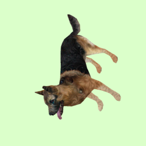
The image synthesis technique is tuned to minimize perceptual perturbations, but does impart a recognizable texture to the objects in the image. This was especially problematic in examples where the original image and the target class were semantically related, or had a similar texture, for example
A dog_191, whose adversarial target was “airedale”
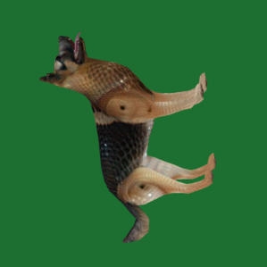
In others, the texture was so obvious that it is no longer visually undetectable.
Dog 63, whose adversarial target was “indian cobra.”
e7_acc_total <- sum(expt_7$correct)/nrow(expt_7)Overall summary
e4_image$meanrt <- NA
e5_image$meanrt <- NA
e6_image$meanrt <- NA
e7_image$meanrt <- NA

e5_sub <- e5_image[,-c(5,6,7,8)]
e3a_accs <- adjusted_accuracy(e3a_image, e3a_subject, level=1/48)
e3b_accs <- adjusted_accuracy(e3b_image, e3b_subject,level=1/48)
all_images <- bind_rows("expt_1"=e1_accs,
                    "expt_2"=e2_accs,
                    "expt_3a"=e3a_accs,
                    "expt_3b"=e3b_accs,
                    "expt_4"=e4_accs,
                    "expt_5"=e5_accs,
                    "expt_6"=e6_accs,
                    "expt_7"=e7_accs,
                    .id="expt")

all_images$reported_img <-     c(94, 71, 79, 81, 100, 73, 100, 78)
all_images$reported_subject <- c(98, 91, 88, 90, 81,  89, 87,  83)

all_im_melt <- reshape2::melt(all_images, measure.vars=c("image", "subject", "reported_img", "reported_subject"))

all_im_melt$type <- "image"
all_im_melt[all_im_melt$variable %in% c("subject", "reported_subject"),]$type <- "subject"

all_im_melt$which <- "adjusted"
all_im_melt[all_im_melt$variable %in% c("reported_subject", "reported_img"),]$which <- "reported"

all_im_melt$expt <- ordered(all_im_melt$expt, levels=experiment_names)
all_im_melt$type <- ordered(all_im_melt$type, levels=c("image", "subject"))
all_im_melt$which <- ordered(all_im_melt$which, levels=c("reported", "adjusted"))

all_im_melt$which_type <- paste(all_im_melt$type, all_im_melt$which)
all_im_melt$which_type <- ordered(all_im_melt$which_type, levels=c("image reported", "subject reported", "image adjusted", "subject adjusted"))ggplot(all_im_melt, aes(x=expt, y=value,
fill=which_type))+
geom_col(position="dodge")+
scale_fill_brewer(palette="Paired")+
theme(axis.text.x=element_text(angle=45,hjust=1))